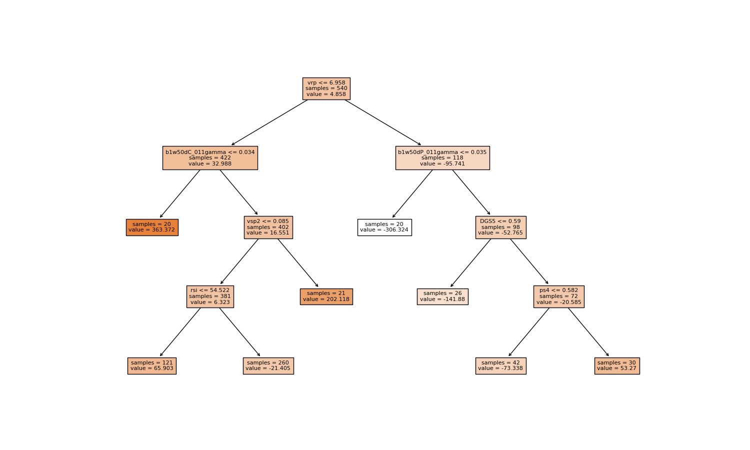
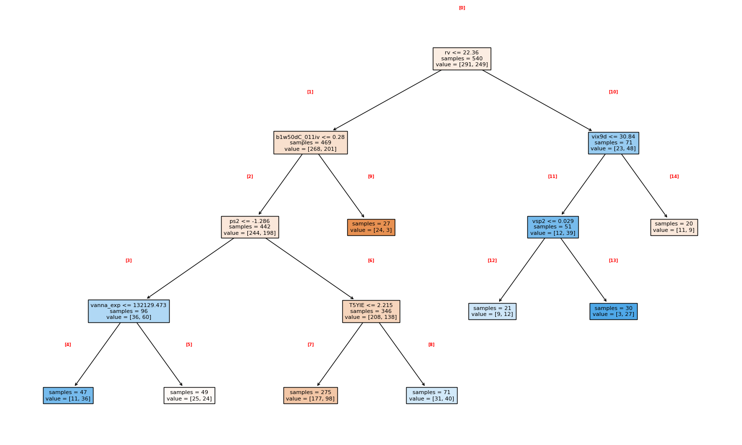
Data Preprocessing:
Convert continuous Y values [10, 20, 30, 40, 50] into categorical classes: ["low", "low", "medium", "high", "high"]
•
Original Gini impurity from all Y classes
•
For each feature
•
For each possible split (based on X values)
•
Split Y classes into two groups
•
Calculate class frequencies and Gini impurity for each group
•
Combine Gini impurities with weighted average
•
Information Gain = Original Gini - Weighted Gini
•
Track split with highest gain for this feature
•
Select best split across all features
After finding the best split:
Create the split
Use the best split to divide the data into two child nodes
Recursively repeat the process
On each child node:
• For the left child, find the best split among all its data points
• For the right child, find the best split among all its data points
• Each child becomes a new decision node with its own best split
Continue until stopping criteria are met
• Maximum depth reached
• Minimum samples per leaf reached
• Information gain below threshold
• Node becomes "pure enough"
Create leaf nodes
When splitting stops, the node becomes a leaf that predicts the most frequent class of all Y values in that node
Prediction Example:
New data point: X₁=4, X₂=7
Tree navigation:
• Root: "X₁ < 5?" → YES (4 < 5) → go left
• Left node: "X₂ < 6?" → NO (7 ≥ 6) → go right
• Right node: LEAF → contains training Y classes ["low", "medium", "low"]
• Prediction: class = "low" (most frequent)
Decision Tree Split Analysis - Classifier
Data Preprocessing
Convert continuous Y values [10, 20, 30, 40, 50] into categorical classes: ["low", "low", "medium", "high", "high"]
Original Gini Impurity
Feature X values: [1, 3, 5, 7, 9]
All Y classes: ["low", "low", "medium", "high", "high"]
Class frequencies: "low"=2, "medium"=1, "high"=2
Class probabilities: P("low")=2/5, P("medium")=1/5, P("high")=2/5
Gini = 1 - (2/5)² - (1/5)² - (2/5)² = 1 - 0.16 - 0.04 - 0.16 = 0.64
Split 1: X < 1 vs X ≥ 1
Group 1 (X < 1): X = [], Y = [] (empty) → Gini = 0 (undefined/0 by convention)
Group 2 (X ≥ 1): X = [1, 3, 5, 7, 9], Y = ["low", "low", "medium", "high", "high"] → Gini = 0.64
Weighted Gini = (0/5) × 0 + (5/5) × 0.64 = 0.64
Information Gain = 0.64 - 0.64 = 0
Split 2: X < 3 vs X ≥ 3
Group 1 (X < 3): X = [1], Y = ["low"] → Gini = 0
Group 2 (X ≥ 3): X = [3, 5, 7, 9], Y = ["low", "medium", "high", "high"] → Gini = 0.625
Weighted Gini = (1/5) × 0 + (4/5) × 0.625 = 0.5
Information Gain = 0.64 - 0.5 = 0.14
Split 3: X < 5 vs X ≥ 5
Group 1 (X < 5): X = [1, 3], Y = ["low", "low"] → Gini = 0
Group 2 (X ≥ 5): X = [5, 7, 9], Y = ["medium", "high", "high"] → Gini = 0.444
Weighted Gini = (2/5) × 0 + (3/5) × 0.444 = 0.267
Information Gain = 0.64 - 0.267 = 0.373
Split 4: X < 7 vs X ≥ 7
Group 1 (X < 7): X = [1, 3, 5], Y = ["low", "low", "medium"] → Gini = 0.444
Group 2 (X ≥ 7): X = [7, 9], Y = ["high", "high"] → Gini = 0
Weighted Gini = (3/5) × 0.444 + (2/5) × 0 = 0.267
Information Gain = 0.64 - 0.267 = 0.373
Split 5: X < 9 vs X ≥ 9
Group 1 (X < 9): X = [1, 3, 5, 7], Y = ["low", "low", "medium", "high"] → Gini = 0.625
Group 2 (X ≥ 9): X = [9], Y = ["high"] → Gini = 0
Weighted Gini = (4/5) × 0.625 + (1/5) × 0 = 0.5
Information Gain = 0.64 - 0.5 = 0.14
Result
Splits 3 and 4 tie for highest Information Gain (0.373).
The algorithm would choose one of them (often the first encountered).
•
Create N bootstrap samples (with replacement)
•
For each bootstrap sample (in parallel)
•
Original Gini Impurity from Y values in this sample
•
For each node split
•
Randomly select subset of features (√n_features)
•
For each selected feature
•
For each possible split (based on X values)
•
Split Y values into two groups
•
Calculate class counts and Gini for each group
•
Combine Gini scores with weighted average
•
Information Gain = Original Gini - Weighted Gini
•
Track split with highest gain for selected features
•
Select best split and continue building tree
•
Majority vote from all N trees
•
Initialize predictions (class probabilities)
•
For each tree (sequentially)
•
Calculate probability residuals (gradients)
•
Original impurity from residuals (not original Y)
•
For each feature
•
For each possible split (based on X values)
•
Split residuals into two groups
•
Calculate gain metric for each group
•
Combine scores with weighted average
•
Information Gain = Residual impurity - Weighted impurity
•
Track split with highest gain for this feature
•
Select best split across all features
•
Update probabilities += learning_rate × tree_prediction
•
Final prediction = class with highest probability

